Geo Diff 2 Analysis

Geo-diff is a service that processes geospatial data. It is composed of several components, including a RabbitMQ broker, a dealer, an admin worker, and worker nodes. The dealer is responsible for enqueuing tasks, the admin worker is responsible for scaling the worker nodes, and the worker nodes are responsible for processing the tasks.

In this section we analyze the performance of the cluster in AWS. We will conduct several experiments to evaluate the performance of the cluster under different conditions.

More info about the project can be found in the intro post.

Clarifications

During the analysis, when we mention geo-diff-worker, we refer to the worker script running in the stack processing tasks. When we say worker nodes, we refer to the VMs or worker instances within AWS.

Parameters

Again, we define the important parameters of the cluster. In this series of experiments, we maintain the parameters of the admin_worker as the objective, adding those of the dealer.

*The value defined is the default. In this series of iterations, they will vary depending on where, what, and how we test.

In the following experiments, we will focus primarily on these attributes:

• admin_worker.MAX_SCALE
• admin_worker.MIN_SCALE

Additionally, we will slightly vary the following attributes to evaluate performance with the same number of geo-diff-worker

• admin_worker.REFRESH_RATE
• admin_worker.QTY_TASK
• dealer.BATCH
• dealer.WAIT

Why was the dealer included in this study?

This script determines the number of messages per second that will be enqueued in the TASK_QUEUE. By increasing and decreasing both dealer.BATCH and dealer.WAIT, we can increase the input to the cluster and thus increase the processing speed, as long as we don’t collapse the network and the geo-diff-worker nodes.

Amazon EC2 Instance

We use t2.micro instances mainly because of their low cost. For more details on the setup used, see AWS Guide

How do credits work?

T2 instances receive CPU credits continuously at a fixed rate based on the instance size, accumulating CPU credits when they are inactive and consuming them when they are active. These credits can be applied to the bill. However, if the credits run out, additional costs must be paid for the excess.

Types of Hardware for Services

After experiencing the surprise of not being able to deploy the entire stack on a single node (the instance crashed and we had to start over), we defined hardware types to avoid the cluster collapsing during deployment.

version: "3.2"
services:
    rabbitmq-server:
            ...       
            resources:
                limits:
                    cpus: "0.50"
                    memory: 512M
                reservations:
                    cpus: "0.25"
                    memory: 200M

    dealer:
            ...
            resources:
                limits:
                    cpus: "0.30"
                    memory: 200M
                reservations:
                    cpus: "0.05"
                    memory: 30M
    
    updater:
            ...
            resources:
                limits:
                    cpus: "0.30"
                    memory: 200M
                reservations:
                    cpus: "0.05"
                    memory: 20M

    worker:
            ...
            resources:
                limits:
                    cpus: "0.75"
                    memory: 400M
                reservations:
                    cpus: "0.3"
                    memory: 100M

    admin-worker:
            ...
            resources:
                limits:
                    cpus: "0.5"
                    memory: 400M
                reservations:
                    cpus: "0.1"
                    memory: 50M

All these hardware limits and reservations were defined based on execution on localhost (SEE ANALYSIS). They may not be exact but give an idea of the resources that must be present in the cluster at a minimum.

Dataset

We used the provided tiles (TILES), which are around 1.5GB in size. This is a collection extracted from NASA’s API with tiles at a monthly frequency from 2016-01 to 2019-12. Each task executed by the geo-diff-worker generates 3 tiles, so the expected generated data is around ~10GB (a bit more than 8GB after applying resizing and other operations on the images).

Experiments

Experiment 1

In this experiment, we will study how the cluster behaves under the following parameters:

version: "3.2"
services:
    dealer:
        ...
        environment:
            ...
            WAIT: 2
            BATCH: 300
            ...

    admin-worker:
        ...
        environment:
            ...
            QTY_TASK: 1
            REFRESH_RATE: 5
            MIN_SCALE: 8
            MAX_SCALE: 8

In those cases where parameters were not indicated, we will use the default parameters indicated in the Parameters table.

Objective

This first iteration is exploratory; mainly, we will see if it is possible to run the cluster with minimal parameters.

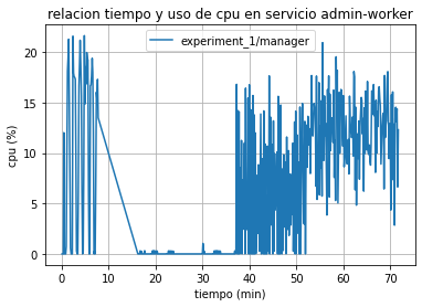
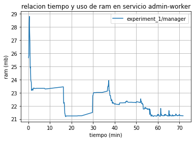
Experiment 1 - Admin Worker

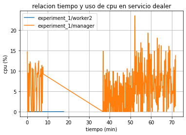
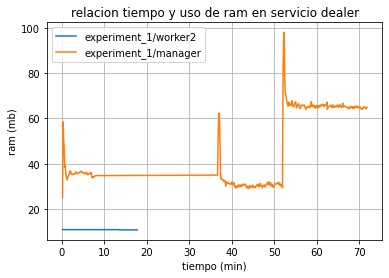
Experiment 1 - Dealer

Experiment 1 - RabbitMQ

Experiment 1 - Updater

Experiment 1 - geo-diff-worker

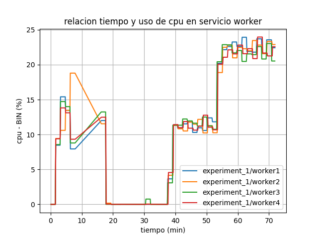
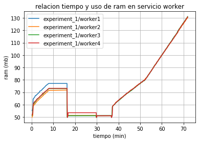
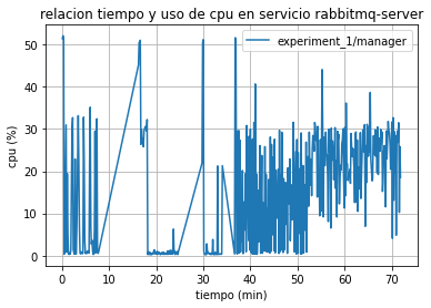
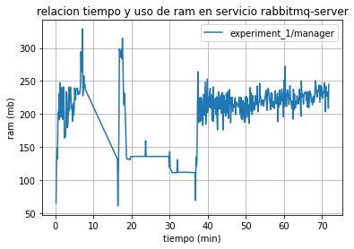
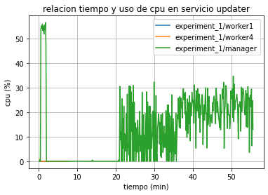
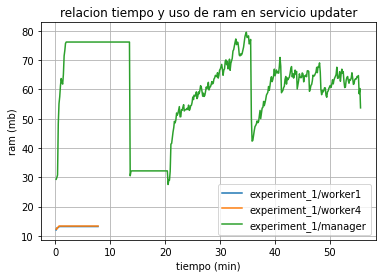
Excellent! We managed to run the entire stack with very good performance. All services are within the expected resource consumption parameters.

Now let’s see how long the geo-diff-worker took to complete the work and how much data was generated.

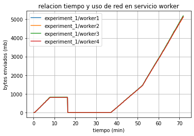
Great! We were in the order of 20GB (5000MB per 4 worker nodes). Note that the graph shows the cumulative amount of bytes sent; at instant 70, ~5000MB had already been sent.

Experiment 2.1

In this experiment, we will study how the cluster behaves under the following parameters:

version: "3.2"
services:
    dealer:
        ...
        environment:
            ...
            WAIT: 2
            BATCH: 300
            ...

    admin-worker:
        ...
        environment:
            ...
            QTY_TASK: 1
            REFRESH_RATE: 2 #
            MIN_SCALE: 12 #
            MAX_SCALE: 12 #

Objective

In this second iteration, we will evaluate the cluster’s performance by scaling the number of geo-diff-worker and the refresh rate (REFRESH_RATE). The main objective is to observe whether 12 is an appropriate number of geo-diff-worker.

Experiment 2.1 - geo-diff-worker

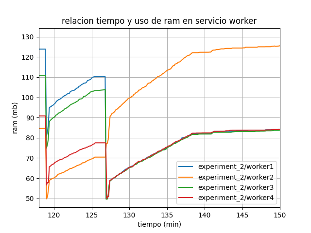
20% CPU is reasonable for the number of available nodes and the time in which the process completed (it took 20 minutes, shown in the graph from minute 120 to 140). We could have increased the number of geo-diff-worker instances a little more, but we risked starving other functionality (for example, being able to SSH into the node to extract execution information).

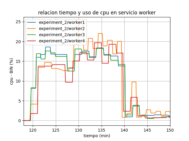
Note: The previous graph has been smoothed by applying an average over groups of 5 samples. Its high variance made it impossible to visualize.

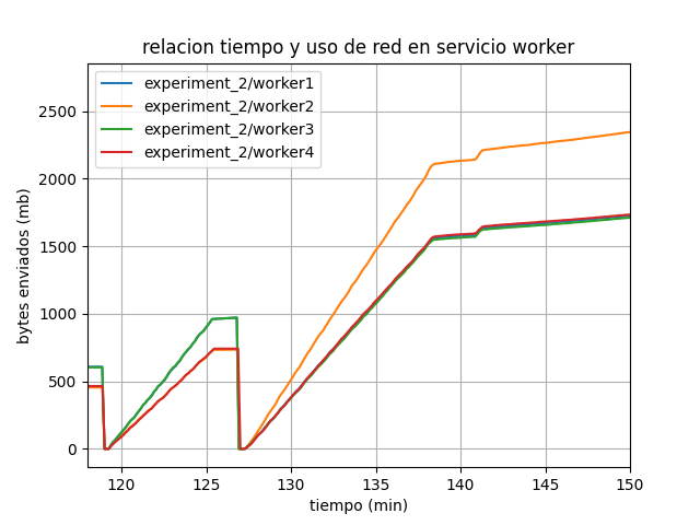
We can observe how the amount of bytes increases, completing the ~10GB (2.5 * 4) of processed tiles that result from the already segmented dataset.

Experiment 2.2

In this experiment, we will study how the cluster behaves under the following parameters:

version: "3.2"
services:
    dealer:
        ...
        environment:
            ...
            WAIT: 2
            BATCH: 600 #
            ...

    admin-worker:
        ...
        environment:
            ...
            QTY_TASK: 1
            REFRESH_RATE: 2
            MIN_SCALE: 12
            MAX_SCALE: 12

Objective

In this iteration, we will study what happens if we modify the dealer.BATCH parameter. We expect the number of tasks to increase and there to be much more network load.

Experiment 2.2 - Dealer

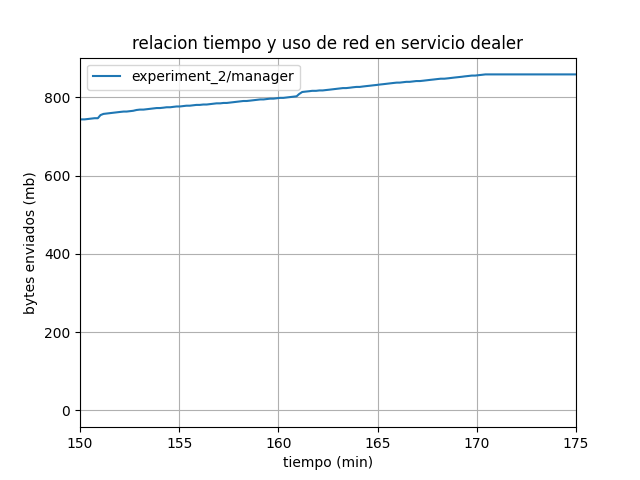
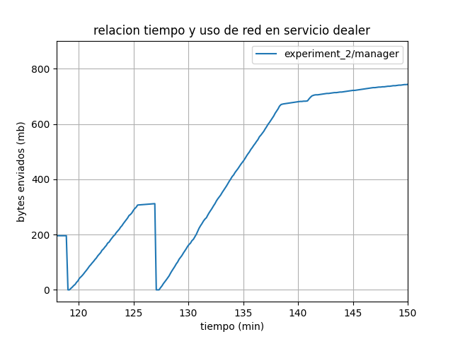
As we can observe, the effect was totally contrary to what was expected; the number of packets sent was lower. It is very possible that this is due to the restrictions we have with the t2.micro machines. For future analyses, we return to the dealer.BATCH value of 300.

Dealer OUT Traffic - Previous Experiment (2.1)

Experiment 2.3

In this experiment, we will study how the cluster behaves under the following parameters:

version: "3.2"
services:
    dealer:
        ...
        environment:
            ...
            WAIT: 2
            BATCH: 600
            ...

    admin-worker:
        ...
        environment:
            ...
            QTY_TASK: 1
            REFRESH_RATE: 0.2 #
            MIN_SCALE: 12
            MAX_SCALE: 12

Objective

In this iteration, we will study how the nodes behave without input. We will try to determine how much CPU% is wasted if there is no load in the cluster, i.e., we will find out if using the admin-worker is useful.

Experiment 2.3 - geo-diff-worker

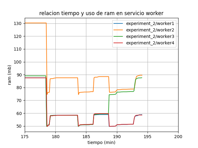
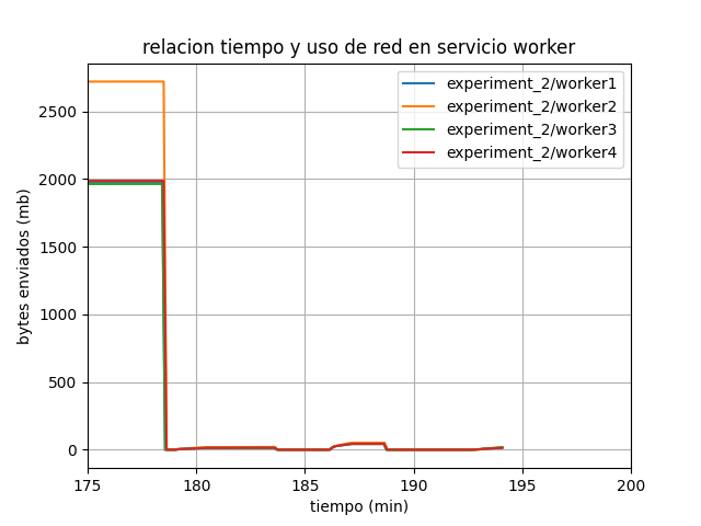
As we said earlier, we observe that the network traffic during this period remains almost null, meaning we effectively have no tasks to perform by the nodes.

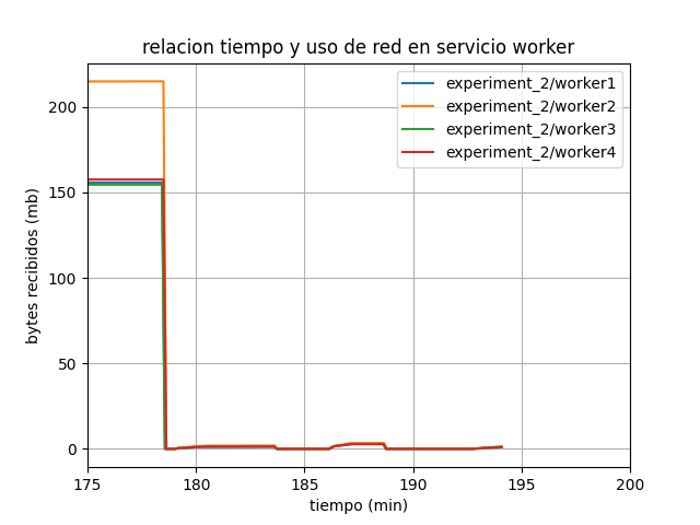
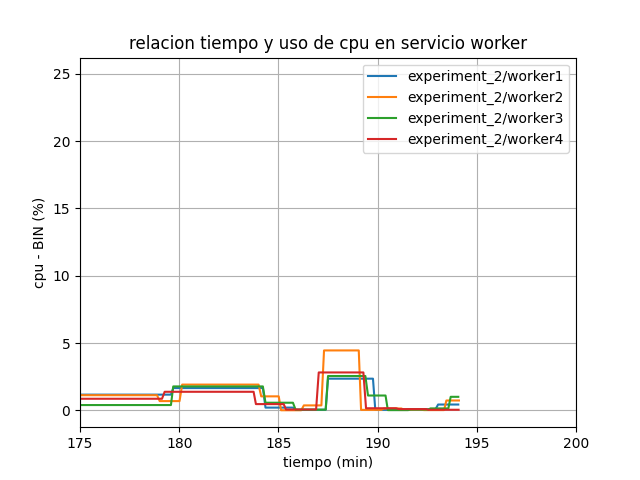
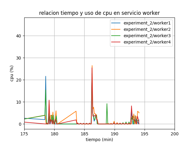
As we can see, we are indeed wasting CPU cycles. It’s not much, but occasionally it reaches 5% usage (and with peaks that exceed 20%, which we can observe in the CPU figure without applying bins).

But, how much are we wasting if we don’t use the autoscaling of geo-diff-worker when the cluster is idle?

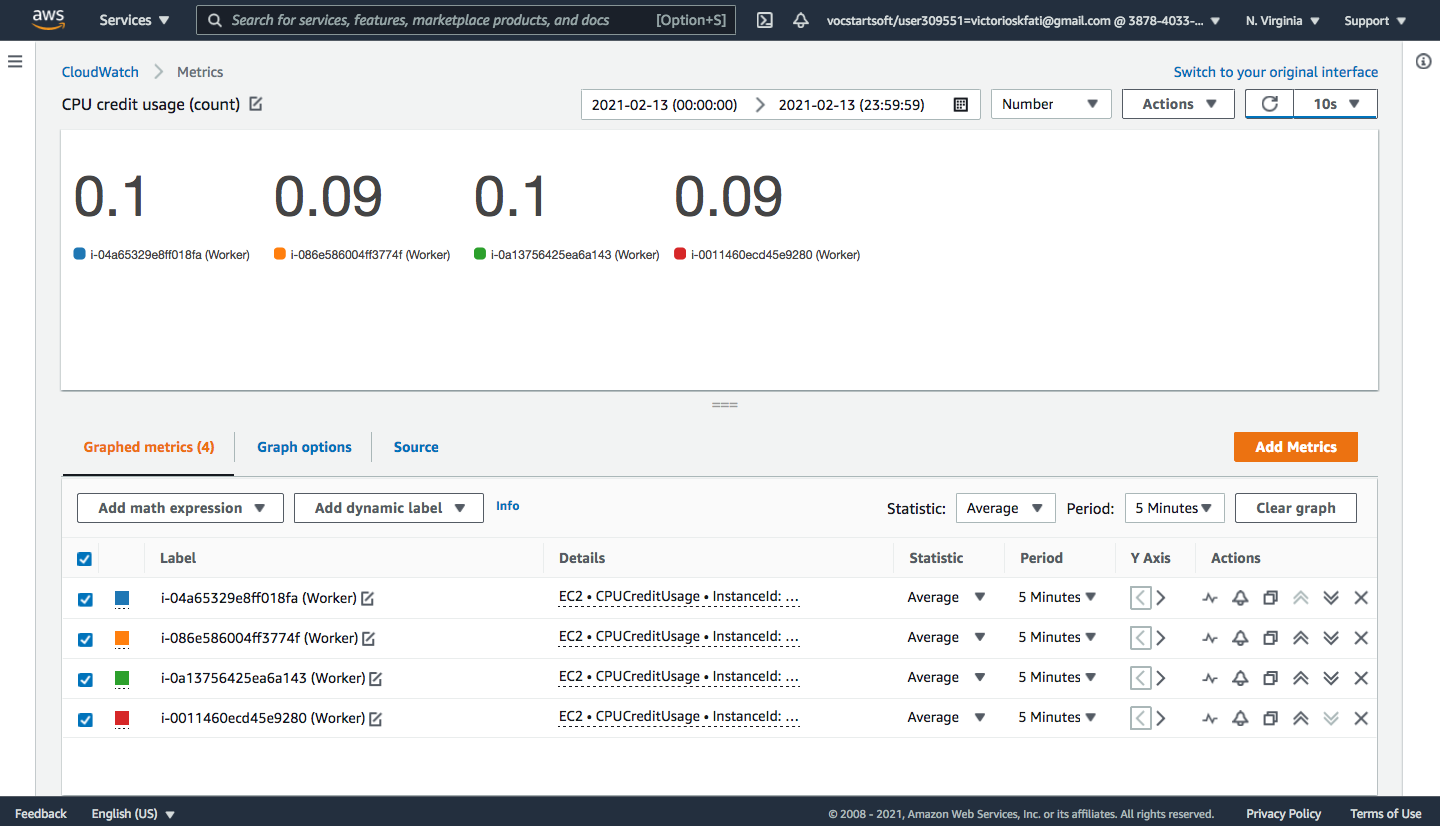
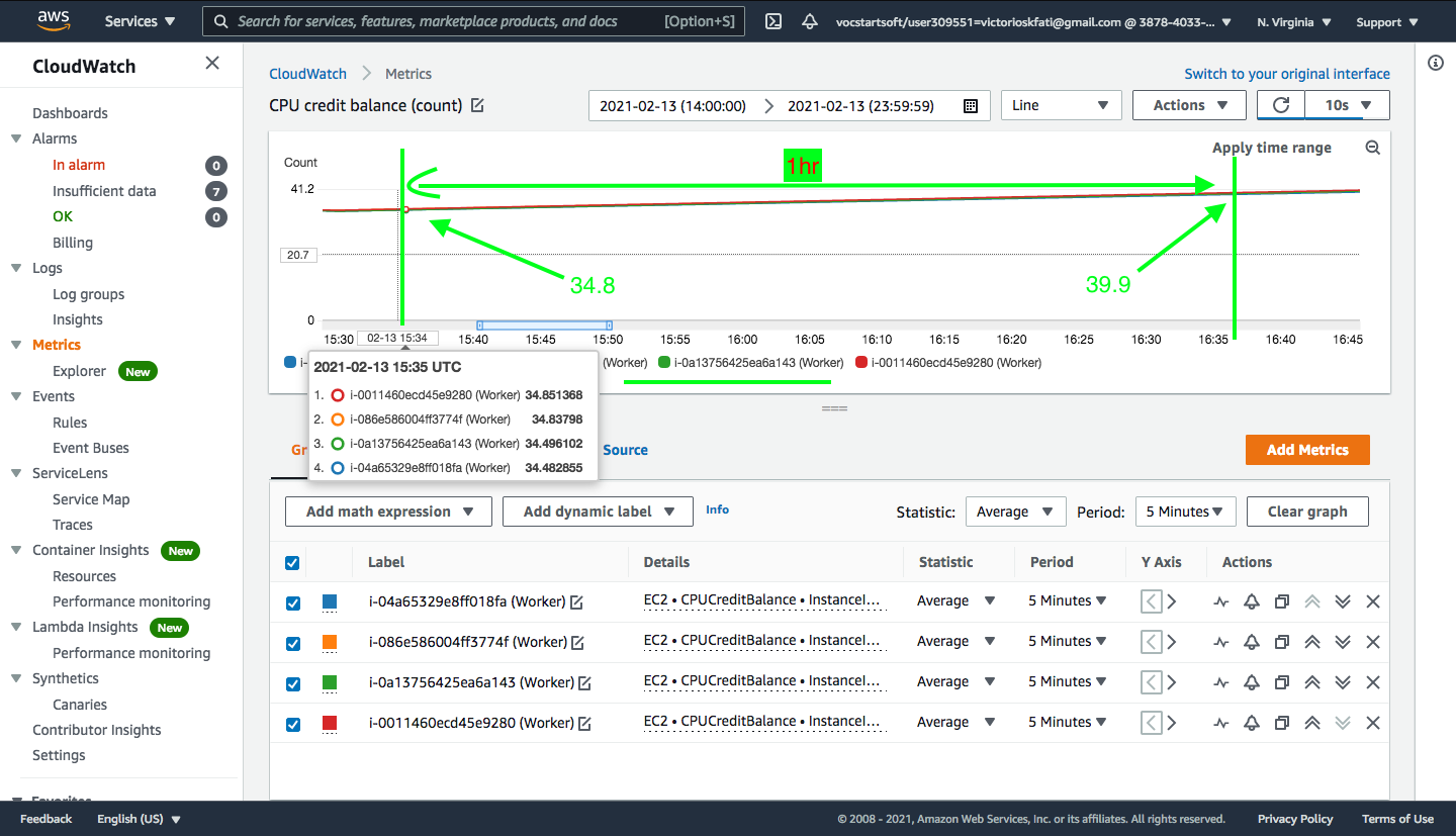
It costs 0.1 credits every 5 minutes (0.1/6 = 1%) per instance. This may seem insignificant, but it’s important to note that running the cluster with load costs ~1 credit every 5 minutes (1/6 = 1%). If we consider that this test lasted ~1 hour, it ended up costing us 5.1 credits per instance (see the figure below), which almost exceeds the 6 credits per instance that we would pay in overages (see Amazon EC2 Instance - How Do Credits Work?).

Experiment 3

In this experiment, we will study how the cluster behaves under the following parameters:

version: "3.2"
services:
    dealer:
        ...
        environment:
            ...
            WAIT: 2
            BATCH: 600
            ...

    admin-worker:
        ...
        environment:
            ...
            QTY_TASK: 15 #
            REFRESH_RATE: 1 #
            MIN_SCALE: 8 #
            MAX_SCALE: 12

Objective

In this iteration, we will evaluate the behavior of the geo-diff-worker under the defined configuration. We expect the cluster to grow and shrink according to the load.

Experiment 3 - Dealer

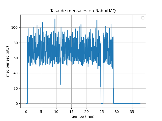
We observe a clear increase in message delivery, with rates ranging from 60-100 per second. These data are extracted from the average publication rate of the TASK_QUEUE queue, from which the geo-diff-worker consumes tasks.

Experiment 3 - Admin Worker

We observe the total cluster load through the admin worker logs. Additionally, we see the number of active geo-diff-worker replicas.

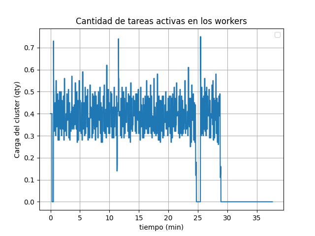
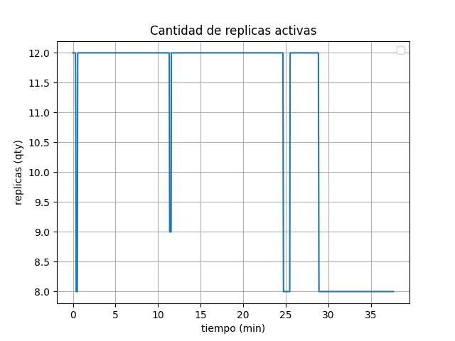
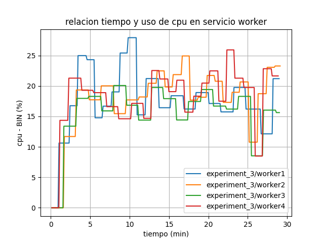
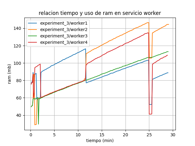
We can see that towards the end, the task load decreases, and therefore geo-diff-worker instances are terminated. If we extrapolate this to memory and CPU consumption (figures in the next section), we can observe that suddenly the RAM/CPU usage drops but then quickly rises again. We suspect this is because the remaining load is distributed among the nodes that remained active, thus increasing both parameters.

Experiment 3 - geo-diff-worker

Experiment 4

In this experiment, we will study how the cluster behaves under the following parameters:

version: "3.2"
services:
    dealer:
        ...
        environment:
            ...
            WAIT: 600 # 10 min
            BATCH: 600
            ...

    admin-worker:
        ...
        environment:
            ...
            QTY_TASK: 15 #
            REFRESH_RATE: 5 #
            MIN_SCALE: 6 #
            MAX_SCALE: 12

Objective

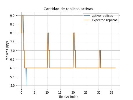
The objective of this last iteration is to distinguish between active and expected replicas. During the previous analysis, we noticed that we were not considering the replicas that were actually running, but only the replicas that should be running. This is because Swarm leaves replicas in a PENDING state if it couldn’t start them, but the counter still remains outdated. Therefore, it was necessary to modify the admin-worker to take the number of active replicas.

After verifying that the replica counter works correctly, we will conduct a final run using 6 to 12 geo-diff-worker instances and increasing the dealer.WAIT parameter to 10 minutes.

Experiment 4 - Admin Worker

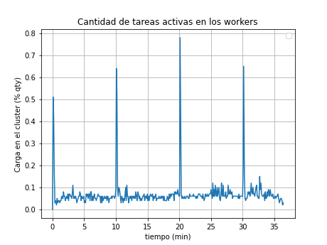
Indeed, we are now seeing the correct number of replicas, and we can observe that it takes a few seconds to update the active replicas (see the graph below). Additionally, we can see that every 10 minutes, the number of tasks increases, so the cluster needs to scale up the number of active replicas.

Experiment 4 - RabbitMQ

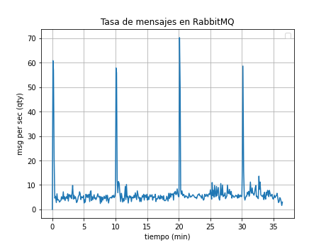
We can observe how every 10 minutes the load in the TASK_QUEUE queue increases.

Experiment 4 - geo-diff-worker

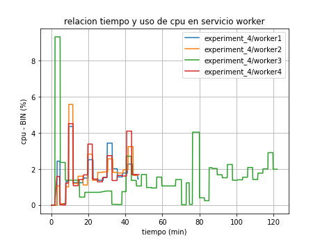
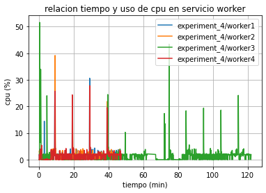
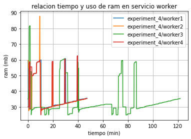
Now we check that the geo-diff-worker instances have been running, and we can see that there were also peaks every 10 minutes or so, moments when the task load increased.

Conclusions

• CPU is what matters. We learned that 5 machines with 1GB of RAM and 1 core perform better than a machine with 8GB and 2 cores.
• Container autoscaling is not a panacea (but we save something). After all, what AWS (and other cloud providers) charge us for are credits per hour of CPU. It’s obvious that deploying containers on demand will reduce the CPU load on idle machines, but the cost of CPU on an idle machine is minimal. The real savings would come from scaling VM instances in the cloud, but for that we have to work much more and migrate to other cluster managers like Kubernetes. Still, the percentage of CPU% saved is high (almost 100% of the credits used without cost, see Experiment 2.3)
• Dockerizing and distributing processes is key. Running this project without Swarm in the cloud would have been almost impossible. We can say that we managed to make the most of the cheapest AWS resources (t2.micro – there are slightly cheaper instances like t2.nano, but they are almost the same as the ones we used, just with less RAM).